Blog

One of the easiest comparison between the influence of coordinate change in general relativity and classical mechanics is the case of acceleration. The case of constant linear acceleration (Rindler coordinates) is fairly well-known, so let's investigate what happens in the rotating case.

We're dealing here with flat spacetime, so our original coordinates are Minkowski space, in cylindrical coordinates to facilitate things later on :

\begin{equation} ds^2 = -dt^2 + dr^2 + dz^2 + r^2 d\theta^2 \end{equation}

The Christoffel symbols are then

\begin{eqnarray} {\Gamma^r}_{\theta\theta} &=& -r\\ {\Gamma^\theta}_{r\theta} &=& \frac{1}{r} \end{eqnarray}

And our geodesic equation is

\begin{eqnarray} \ddot{t} &=& 0\\ \ddot{r} - r \dot{\theta}^2 &=& 0\\ \ddot{z} &=& 0\\ \ddot{\theta} + \frac{2}{r} \dot{r} \dot{\theta} &=& 0 \end{eqnarray}

This is, up to the non-relativistic limit, about what we'd expect from Newton's law in cylindrical coordinates. Now let's consider a rotating frame of reference. Our new coordinates are all identical, except

\begin{equation} \bar{\theta} = \theta - \omega(t) t \end{equation}

with the inverse transformation $\theta = \bar{\theta} + \omega(t) t$. Our derivatives are therefore

\begin{equation} \partial_t \bar{\theta} = - (\omega(t) + \dot{\omega}(t) t),\ \partial_t \theta = \omega(t) + \dot{\omega}(t) t \end{equation}

For now, let's consider $\dot{\omega} = 0$. These are the Born coordinates, and our new metric becomes

\begin{equation} ds^2 = -(1 - \omega^2 r^2) dt^2 + 2 \omega r^2 d\theta dt + dr^2 + dz^2 + r^2 d\theta^2 \end{equation}

The classical equivalent here will be some system rotating with constant velocity. We should then expect two things in the classical limit : the centrifugal force, and the Coriolis force. Our Christoffel symbols become :

\begin{eqnarray} {\Gamma^r}_{\theta\theta} &=& - r\\ {\Gamma^r}_{tt} &=& - r \omega^2\\ {\Gamma^r}_{\theta t} &=& - \omega r\\ {\Gamma^\theta}_{r\theta} &=& \frac{1}{r}\\ {\Gamma^\theta}_{rt} &=& \frac{\omega}{r} \end{eqnarray}

We gain three extra terms related to the rotation. This leads us to the geodesic equations

\begin{eqnarray} \ddot{t} &=& 0\\ r - r \dot{\theta}^2 - 2 \omega r \dot{\theta} \dot{t} - r \omega^2 \dot{t}^2 &=& 0\\ \ddot{z} &=& 0\\ \ddot{\theta} + \frac{2}{r} \dot{r} \dot{\theta} + \frac{2\omega}{r} \dot{r} \dot{t} &=& 0\\ \end{eqnarray}

Now as usual for the non-relativistic limit, we have $t = \beta \tau + t_0$

One of the great forgotten book of general relativity is Synge's "Relativity : The general theory", which opens with the following line

Of all physicists, the general relativist has the least social commitment. He is the great specialist in gravitational theory, and gravitation is socially significant, but he is not consulted in the building of a tower, a bridge, a ship or an aeroplane, and even the astronauts can do without him until they start wondering which ether their signals travel in.

It has so far been the case that, while its effects are measurable, given sufficient precision, general relativity cannot be used for anything particularly practical outside of its classical limit. While quantum field theory can at least have such esoteric use as nuclear reactor detection via neutrino emission, the practical uses of general relativity remain limited.

This has not stopped people from attempting to do it, either theoretically or in practice, as the theory has much to offer at least in principle with its effects, although none of them even close to being feasible, even in laboratory settings. Because of this, it's a domain precariously perched in between speculative ideas and outright quackery. Proceed at your own risks.

Wormholes

The history of wormholes is, depending on what you're willing to consider, quite long, from Flamm's vague sketch of what would one day become the maximally extended Schwarzschild wormhole in 1916, to Reichenbach's discussion of possible topologies of space in 1928, or the famous paper by Einstein and Rosen.

As an engineering idea, though, outside of various science fiction using the idea of the Schwarzschild wormhole directly without too much consideration for the horizon, the common origin of most wormholes is the Morris-Thorne wormhole. Asked by Carl Sagan for a reasonable method of interstellar travel for his novel Contact, Morris and Thorne devised for the first time a spacetime with the express intent of being used for such a purpose, in their 1987 paper, "Wormholes in spacetime and their use for interstellar travel : A tool for teaching general relativity".

Warp drive

A rigorous idea for the warp drive was first formulated only fairly recently, in Alcubierre's 1994 paper, "The warp drive: hyper-fast travel within general relativity".

Anti-gravity

Anti-gravity within the context of general relativity is, at least on a mathematical level, fairly trivial. Depending on your goals for antigravity, either make the metric around an object flat or make your spacetime such that geodesics diverge rather than converge. Unfortunately, from fairly general arguments, we can see that in all likelihood, this is going to mean violating some energy conditions.

For Halloween here is a brief review of the various spooky entities that exist in theoretical physics!

The Ghosts

Ghosts are sort of a catch-all term for unphysical objects in various theories. In particular, the Faddev-Popov ghosts.

In BRST quantization, Fadeev-Popov ghosts

Phantom fields

Phantom fields are a variety of fields for which the kinetic energy is negative

The Demons

Demons refer to a variety of physically-violating entities mostly used in thought experiments. The two most famous ones being Laplace's demon and Maxwell's demon.

Laplace's demon is an entity which

Yet another type of demon in physics appears in the context of the Cauchy problem.

The djinns

Noether's theorem relating continuous Lie symmetries to conserved quantities famously implies that given a time translation symmetry

\begin{equation} \phi(t, x^i) \to \phi'(t) = \phi(t + T, x^i) \end{equation}

with infinitesimal action

\begin{equation} \delta \phi = \varepsilon \dot{\phi} \end{equation}

The Lagrangian density changes by

\begin{eqnarray} \delta \mathcal{L} &=& \frac{\partial \mathcal{L}}{\partial \phi} \varepsilon \dot{\phi} + \frac{\partial \mathcal{L}}{\partial \dot{\phi}} \varepsilon \ddot{\phi}\\ &=& \varepsilon \frac{d}{dt} \mathcal{L} \end{eqnarray}

...

The hidden assumption here is that the field has the proper values and variation on the boundary. If we forgo this condition, energy is not conserved. There are two ways we could break this condition.

The first one is to have an extra boundary to the manifold. This will usually correspond to the condition of a naked singularity in our spacetime. The simplest possible example is to consider the static spacetime made from the slice $\mathbb{R}^3 \setminus \{ 0 \}$, Minkowski space minus the origin.

A good way to convince yourself is to first consider Minkowski space with the charge distribution

\begin{equation} j^\mu(x) = (\theta(t) \delta(x^i), 0) \end{equation}

This is not a very good charge distribution (it has a discontinuous total charge), but this won't matter much. Using the Lorenz gauge, the Maxwell equation is then

\begin{eqnarray} \Box A^0 &=& \theta(t) \delta(x^i)\\ \Box A^i &=& 0 \end{eqnarray}

The exact set of solutions doesn't matter too much here, we are only after a particular one. The simplest will be to assume $A_i = 0$, and using the retarded D'Alembert green function,

\begin{eqnarray} A^0 &=& \int d^4x \theta(t) \delta(x^i) \frac{\delta((t - t_0) + |x^i - x^i_0|)}{4\pi |x^i - x^i_0|}\\ &=& \int dt \theta(t) \frac{\delta(t - (t_0 - |x^i_0|)}{4\pi |x^i_0|}\\ &=& \theta(t_0 - r_0) \frac{1}{4\pi r} \end{eqnarray}

So that, for $r > t$, the potential is the Coulomb potential and simply $0$ otherwise. The electric field $E^i = - \nabla^i A^0$ is then

\begin{eqnarray} E^i &=& -\nabla^i (\theta(t - r) \frac{1}{4\pi r})\\ &=& -\frac{1}{4\pi r} \nabla^i \theta(t - r) - \theta(t - r) \nabla^i \frac{1}{4\pi r}\\ &=& -\frac{x^i}{4\pi r^2} (\delta(t - r) - \theta(t - r) r^{-1}) \end{eqnarray}

The energy of our electric field is then

\begin{eqnarray} H &=& \int E^i E_i d^3x\\ &=& -\int \frac{1}{4\pi r} (\delta(t - r) + \theta(t - r) r^{-1}) d^3x\\ &=& 4\pi \int \frac{r}{4\pi} (\delta(t - r) + \theta(t - r) r^{-1}) dr\\ &=& 4\pi (\frac{t}{4\pi} + \ldots) \end{eqnarray}

Due to their peculiarities, texts on wormholes can pop up in rather mysterious places outside of dry theoretical physics papers, from NASA's Frontiers of Propulsion Science to weird government reports to UFO enthusiasts, all with varying degrees of rigor. While physics papers are easy enough to find electronically, as we've had the use of arxiv for about thirty years, and generally a better access to the older papers as well, those other papers can be somewhat more challenging to find.

Somewhat on the more reasonable side of that scale is the Journal of the British Interplanetary Society. Here we find two papers which are sometimes referred to elsewhere : "Interstellar Travel through Magnetic Wormholes" by Claudio Maccone (vol. 48, pp. 453-458, 1995) and its rebuttal, "“Magnetic Wormholes” and the Levi-Civita Solution to the Einstein Equation" (vol. 50, pp. 155-157, 1997). Neither of these are available electronically, not even on request, nor can they be purchased. But if you ask nicely enough and leave some donation to the society of the appropriate value, someone may photocopy it for you.

I thought that therefore it may be a good idea to put this up here for posterity, in case someone needs to know what the magnetic wormhole is and why it does not work.

First, we need to look at the Levi-Civita spacetime. While indeed discovered by Levi-Civita, in some untranslated Italian paper (recently translated here), it is more commonly known under its modern name of the Bertotti-Robinson spacetime, as it was later on studied by Bertotti and Robinson's A solution of the Einstein-Maxwell equations (Bull. Acad. Polon. Sci. Math. Astron. Phys. 7, 351), itself apparently not available online. It's not the most popular of metrics to study, although it is discussed in Pauli's Theory of relativity (p. 171-172) and of course, Stephani et al.'s Exact Solutions of the Einstein Field Equations (section 12.3).

The Bertotti-Robinson spacetime's basic idea is quite simple, it is a spacetime with a constant electromagnetic field upon it. What it means for the EM field to be constant isn't quite trivial since the EM tensor components will depend on the coordinates, but we'll see what it means later on. As can be guessed from the definition, the Bertotti-Robinson spacetime is an electrovacuum solution, which solves the Einstein-Maxwell equations

\begin{equation} R_{\mu\nu} - \frac{1}{2} g_{\mu\nu} R = (F_{\mu\sigma} {F_{\nu}}^\sigma - \frac{1}{4} g_{\mu\nu} F_{\rho\sigma} F^{\rho\sigma}) \end{equation}

The stress-energy tensor can be shown to be traceless, as the electromagnetic tensor itself is, leading to $R = 0$, so that

\begin{equation} R_{\mu\nu} = (F_{\mu\sigma} {F_{\nu}}^\sigma - \frac{1}{4} g_{\mu\nu} F_{\rho\sigma} F^{\rho\sigma}) \end{equation}

\begin{equation} x \end{equation} ...

There are two invariants of the EM field we can consider to define it as constant,

\begin{eqnarray} I &=& F_{\mu\nu} F^{\mu\nu}\\ J &=& \varepsilon^{\mu\nu\rho\sigma} F_{\mu\nu} F_{\rho\sigma} \end{eqnarray}

As these are scalars, they can be used to define some notion of constant field independently of the coordinates. In flat space they roughly correspond to the quantities $-(\| \vec{E} \|^2 - \| \vec{B} \|^2)$ and $-(\vec{E}\cdot\vec{B})$ (up to some factors), and we therefore say that if $J = 0$ and $I \neq 0$, then either $I < 0$ and the field is electrostatic, or $I > 0$ and the field is magnetostatic (as in, some observers will measure such a field).

...

There are many forms of the Bertotti-Robinson metric

\begin{equation} ds^2 = \frac{1}{\lambda^2 r^2} (-dt^2 + dr^2 + r^2 d\theta^2 + r^2 \sin^2(\theta) d\phi^2) \end{equation} \begin{equation} ds^2 = - \lambda^2 (\rho^2 + z^2) dt^2 + \frac{1}{\lambda^2 (\rho^2 + z^2)} (d\rho^2 + dz^2 + \rho^2 d\theta^2) \end{equation}

A rather tedious task in general relativity is the computation of the various tensor quantities. While there are no general methods to make this task easier (except of course for the use of numeric methods), given metrics of specific properties, it is possible to simplify it greatly.

For a start, a fairly well-known property is the fact that given a diagonal metric, its inverse metric is simply its inverse, component-wise.

$$g^{ab} g_{ac} = \delta^b_c \to g^{aa} g_{aa} = 1 \to g^{aa} = (g_{aa})^{-1}$$

Now, given a diagonal metric, let's consider the Christoffel symbols :

$${ \Gamma^a }_{bc} = \frac{1}{2} g^{ad} (g_{db,c} + g_{dc,b} - g_{bc,d})$$

Then, for a given coordinate $a = x$, we have

$${ \Gamma^x }_{bc} = \frac{1}{2} g^{xx} (g_{xb,c} + g_{xc,b} - g_{bc,x})$$

The first two terms are only non-zero if $b$ or $c$ are equal to $x$, and the last term only if $b = c$. This means that the only type of symbols we have are

\begin{eqnarray} { \Gamma^x }_{bb} &=& -\frac{1}{2} g^{xx} g_{bb,x} & (b \neq x)\\ { \Gamma^x }_{bx} &=& \frac{1}{2} g^{xx} g_{xx,b} &(b \neq x)\\ { \Gamma^x }_{xx} &=& \frac{1}{2} g^{xx} g_{xx,x} \end{eqnarray}

If both $b$ and $c$ are different from $x$ and each other, the symbol will be zero. For a given $x$, there are $(n-1)$ symbols of the first kind, $(n-1)$ of the second kind, and $1$ of the third kind. This reduce the number of symbols from $n^2 (\frac{n + 1}{2})$ to $n (2n-1)$, or for instance, in $4$ dimensions, from $40$ components to $28$.

We can also note some similarities between the different symbols. That is,

$${ \Gamma^x }_{bb} = - \frac{g^{bb}}{g^{xx}} { \Gamma^b }_{bx} = - \frac{g_{xx}}{g_{bb}} { \Gamma^b }_{bx} $$

Occasionally, we find that the metric has the property that, in addition to being diagonal, every component is independent from the coordinate involved. That is, given a coordinate $x$, we have $g_{xx,x} = 0$ (This does not mean that the metric doesn't depend on that coordinate in other components). This is for instance true of the Morris-Thorne metric :

$$ds^2 = -f(l) dt^2 + dl^2 + r^2(l) (d\theta^2 + \sin^2(\theta) d\varphi^2)$$

In this case, things simplify further to just the first and second kind of symbols, leaving only $2n(n-1)$ symbols (or $24$ in $4$ dimensions).

While not the actual definition of symmetry, it is very common for metrics to be completely independent of a coordinate, ie, $g_{ab,x} = 0$. There are up to $n$ such symmetries at most, and given a diagonal metric, this leads to, for $x$ a symmetry, the Christoffel symbols of the first and third type to be zero, as well as those of the second type for when $b$ is such a coordinate. We then get, for $p$ such symmetries, that there are $n(n-p)$ symbols of the first type, $n(n-p)$ of the second type, and $(n-p)$ of the third type, for a total of $(2n+1)(n-p)$. This indeed leads to $0$ symbols for $n = p$ (which is simply Minkowski space).

We can indeed check that, for the Morris-Thorne metric, where we have $p = 2$ (the metric is independant from $t$ and $\varphi$), we have up to $18$ components (actually less so than that due to the lack of dependence on $\varphi$ for most components).

Another property one may encounter from the metric is if it is both diagonal, has a symmetry $g_{ab,x} = 0$, and is such that $g_{xx,a} = 0$ for every coordinate $a$. This is for instance true of the Ellis-Bronnikov metric

$$ds^2 = -dt^2 + dl^2 + (l^2 + a^2) (d\theta^2 + \sin^2 \theta d\varphi^2)$$

where this is true for the coordinate $t$. In such a case, for $x$ the symmetry, we have that all three types of symbols are zero, which gets rid of quite a lot of components (at this point the spacetime is basically a trivial warped product $ds^2 = dx + h$, and we simply need to get the connection components of the metric $h$, similarly to what happens for ultrastatic spacetimes).

Once we have those symbols, we can tackle the Riemann tensor

$${R^a}_{bcd} = {\Gamma^a}_{bd,c} - {\Gamma^a}_{bc,d} + {\Gamma^a}_{ce} {\Gamma^e}_{bd} - {\Gamma^a}_{de} {\Gamma^e}_{bc}$$

Due to its symmetries, there are

$$C_n = \frac{1}{12} n^2(n^2 - 1)$$

independent components. There again, we can use properties from the metric to reduce the number of components to compute.

$${R^x}_{bcd} = {\Gamma^x}_{bd,c} - {\Gamma^x}_{bc,d} + {\Gamma^x}_{ce} {\Gamma^e}_{bd} - {\Gamma^x}_{de} {\Gamma^e}_{bc}$$

Here's a list of proofs of Geroch's quiz on spacetimes from the previously mentionned paper. Most of which done using counterexamples. For a brief reminder :

Take all spacetimes to be four-dimensional, and, for assertions involving causal structure, time-oriented. All manifolds are to be Hausdorff, paracompact, connected, and without boundary.

1. A manifold admits a Lorentz metric if and only if its universal covering manifold does. (FALSE)

As is well known (from the mysterious proof of Steenrod's Topology of fiber bundles), given Geroch's definition of a manifold, there's only one case for which a manifold may fail to admit a Lorentz metric : if it is both compact and has an Euler characteristic different from zero. So what we are looking for is a compact manifold of non-zero Euler characteristic which has a universal cover that either does not, or is non-compact.

A very simple example is the surface of genus two $S_2 = T^2 \# T^2$, which has Euler characteristic $2$, but has the hyperbolic plane $\mathbb{H}^2$ as its universal cover, which is non-compact. But for our case, we have to assume $4$-dimensional manifolds. Fortunately, as the covering space of a product of spaces is the product of their respective covering spaces, we have that the product of two such surfaces $S_2 \times S_2$ (with Euler characteristics $\chi(S_2 \times S_2) = \chi(S_2) \times \chi(S_2) = 4$) is $\mathbb{H}^2 \times \mathbb{H}^2$, also non-compact. Hence we have a proper counterexample.

2. Every flat spacetime admits a nonzero Killing field. (FALSE)

Not to get confused (this wouldn't work with some notion based on local properties like simply a vector field obeying the Killing equation), let's have a quick reminder of what a Killing vector field is :

Given Minkowski space, we have the full Poincaré group as the set of all isometries on the manifold. A simple way of removing those isometries is by simply removing points : removing a single point from the manifold, all translation isometries already vanish (for instance removing $0$, the translation isometries of $x,y,z$ with parameter $t = 1$ no longer work for $(-1,0,0)$, $(0,-1,0)$, and $(0,0,-1)$). For $4$ dimensions, we simply have to remove a point along every axis as well to prevent rotational Killing vector fields.

3. Call two Lorentz metrics on M equivalent if there is a diffeomorphism from M to M which sends one to the other. Then each of two equivalent metrics can be continuously deformed to the other. (FALSE)

4. For $M$ a, a manifold, and $p$, a point of $M$, $M$ with $p$ removed is not diffeomorphic with $M$. (FALSE)

The counterexample is fairly simple to come up with once you realize that the big obstacle is just the lack of bijections between two finite sets of different cardinalities. Just have the manifold already contain a countable infinity of points removed :

$$M = \mathbb{R}^4 \setminus \{ (t,x,y,z) | t = y = z = 0 \wedge x \in \mathbb{N}_{> 0} \}$$

Then simply remove $(0,0,0,0)$, $M' = M \setminus \{ (0,0,0,0) \}$. The diffeomorphism $\phi : M \to M'$ is then just

$$\phi(t,x,y,z) = (t,x-1,y,z)$$

5. If spacetime $M, g_{ab}$ has vanishing Weyl tensor, then $\Omega^2 g_{ab}$ is flat for some $\Omega$. (FALSE)

6. If, for $C$ a closed subset of $M$, $M \setminus C$ admits a Lorentz metric, then so does $M$. (FALSE)

Fairly easy to do by considering the usual counterexample of Lorentzian manifolds : $S^2$ minus a disk is homeomorphic to $\mathbb{R}^2$, and the same is true of $S^4$ and $\mathbb{R}^4$. As $S^4$ admits no Lorentz metric, this is false.

7. For $S$, a two-dimensional manifold, and $p$, a point of $S$, $S \setminus p$ is not simply connected. (FALSE)

Consider $S^2$ for the manifold, $S^2 \setminus \{ p \} \cong \mathbb{R}^2$, which is simply connected.

8. The product of two simply connected manifolds is simply connected. (TRUE)

From standard results, we have that $\pi_1(X \times Y) = \pi_1(X) \times \pi_1(Y)$, so that in our case, the product of the trivial groups $\{ i_X \}$ and $\{ i_Y \}$ is the also trivial group $\{ (i_X, i_Y) \}$.

9. If, for $S$ and $S'$, three-dimensional manifolds, $S \times \mathbb{R}$ and $S' \times \mathbb{R}$ are diffeomorphic then $S$ and $S'$ are diffeomorphic. (FALSE)

Not a whole lot of simple counterexamples unfortunately, but it is famously true of the Whitehead manifold.

10. No compact spacetime is extendible. (TRUE)

If a compact manifold $M$ is extendible, there exists some inclusion $\iota : M \to M'$, $M'$ some connected manifold, such that $\iota(M) \neq M'$, and where $\iota(M)$ is an open submanifold isometric to $M$. From the isometry, $\iota(M)$ is compact and therefore closed. It is therefore closed and open, which means that since $M'$ is connected, it can only be $M'$ or $\varnothing$.

11. Every simply connected $4$-manifold which is a product admits a Lorentz metric, except $S^2 \times S^2$. (TRUE)

While $4$-manifolds aren't so easily classified, things are much simpler in this case. We can only consider the following two cases : either the product of two $2$-manifolds, or the product of a $3$-manifold with a $1$-manifold (the case of four $1$-manifolds can be reduced to either).

From the product property of the fundamental group, if the $4$-manifold is simply connected, then so are its components here. And the same is true of compactness : it will only be compact if both are. This simplifies things considerably : $\mathbb{R}$ is not compact and $S$ is not simply connected, hence we can only have the product of two $2$-manifolds. Of these, only the sphere is both compact and simply connected, from the usual theorem of classification of surfaces. Hence this statement is correct.

12. A spacetime is extendible if and only if its universal covering spacetime is. (FALSE)

13. A non-simply connected manifold which admits a Lorentz metric admits one which is neither time-orientable nor space-orientable. (FALSE)

14. A flat spacetime is time-orientable. (FALSE)

A seldomly brought up theorem is that, given a spacetime of the form $\mathbb{R} \times \Sigma$, $\mathbb{R}$ being a timelike coordinate and $\Sigma$ a spacelike hypersurface, and considering the time-reversal operator $T(t, \sigma) = (-t, \sigma)$ and some involution $I$ on $\Sigma$, then $(\mathbb{R} \times \Sigma) / (T \times I)$ fails to be time-orientable (this can be checked by considering some closed curve passing through two points $p, q \in \mathbb{R} \times \Sigma$ such that $p \sim q$ and checking what happens to a timelike vector transported on it).

Given this, a simple example of a flat non-time-orientable spacetime is the Minkowski cylinder $\mathbb{R} \times S$,

$$ds^2 = -dt^2 + d\theta^2$$

with the involution $I(t,\theta) = (t, \theta + \pi)$.

15. If each of two spacetimes can be embedded isometrically as an open subset of the other, then the spacetimes are isometric. (FALSE)

An example of such a pair of spacetimes is to consider two upper half Minkowski planes, $\mathbb{R}^2_{t > 0}$, but the second one has a point $(t_1, x_1)$ removed. Then we can consider the isometry of simply the identity map with a point removed for going from the first to the second, and the identity translated by $t_1$ for the second to the first.

This theorem is also apparently true if the manifolds are compact and oriented.

16. The sum of two complete vector fields is complete. (FALSE)

One of my favorite GR paper is "Global structure of spacetimes", by Robert Geroch and Gary Horowitz, included in Hawking and Israel's "General relativity : an Einstein centenary survey". It contains quite a few proofs and ideas rarely repeated elsewhere, as well as the following few interesting passages :

First : a brief description of the general methods used for proofs in the study of spacetime global structures in the paper :

The role of key theorems has been assumed instead by 'methods of proof', for indeed there are a limited number of these, which do occur over and over. In fact, the following eight methods of proof will suffice for most results in this subject : 'Introduce a timelike vector field (and, usually, then consider its integral curves)', 'Carry information about closed curves and compare with what one had at the beginning', 'Connect timelike or null curves together, and smooth the corners, to obtain new curves', 'Find a sequence of points with some property and ask for an accumulation point', 'Choose a sequence of points which approach the point in question (usually from a timelike direction) and try to carry some property to the limit', 'Ask for the timelike curve of maximal length between two points, or between a point and a surface', 'Take the domain of dependence, and study the Cauchy horizon', and 'Find a sequence of timelike curves with some property, and ask for an accumulation curves'.

General tips for constructing spacetime examples :

The examples, although they are particularly numerous in this subject, are in practice rather easy to obtain. Indeed, the following seven techniques (or, more often, combinations of two or more) will normally produce the desired example : 'Check the known solutions', 'Tip the light-cones in some way', 'Take a covering space or product', 'Isolate what makes an example fail in a local region, and push that region off to infinity', 'Introduce a conformal factor', 'Patch spacetimes together across boundary surfaces' and 'Cut holes of various types in given spacetimes'.

And this heap of random theorems presented without proofs as a quiz (Answers included):

Prove or find a counterexample to the following assertions. Take all spacetimes to be four-dimensional, and, for assertions involving causal structure, time-oriented. All manifolds are to be Hausdorff, paracompact, connected, and without boundary.

Manifolds, metrics, orientation

1. A manifold admits a Lorentz metric if and only if its universal covering manifold does. (FALSE)
2. Every flat spacetime admits a nonzero Killing field. (FALSE)
3. Call two Lorentz metrics on $M$ equivalent if there is a diffeomorphism from $M$ to $M$ which sends one to the other. Then each of two equivalent metrics can be continuously deformed to the other. (FALSE)
4. For $M$ a, a manifold, and $p$, a point of $M$, $M$ with $p$ removed is not diffeomorphic with $M$. (FALSE)
5. If spacetime $M, g_{ab}$ has vanishing Weyl tensor, then $\Omega^2 g_{ab}$ is flat for some $\Omega$. (FALSE)
6. If, for $C$ a closed subset of $M$, $M \setminus C$ admits a Lorentz metric, then so does $M$. (FALSE)
7. For $S$, a two-dimensional manifold, and $p$, a point of $S$, $S \setminus p$ is not simply connected. (FALSE)
8. The product of two simply connected manifolds is simply connected. (TRUE)
9. If, for $S$ and $S'$, three-dimensional manifolds, $S \times \mathbb{R}$ and $S' \times \mathbb{R}$ are diffeomorphic then $S$ and $S'$ are diffeomorphic. (FALSE)
10. No compact spacetime is extendible. (TRUE)
11. Every simply connected $4$-manifold which is a product admits a Lorentz metric, except $S^2 \times S^2$. (TRUE)
12. A spacetime is extendible if and only if its universal covering spacetime is. (FALSE)
13. A non-simply connected manifold which admits a Lorentz metric admits one which is neither time-orientable nor space-orientable. (FALSE)
14. A flat spacetime is time-orientable. (FALSE)
15. If each of two spacetimes can be embedded isometrically as an open subset of the other, then the spacetimes are isometric. (FALSE)
16. The sum of two complete vector fields is complete. (FALSE)

Domain of influence

17. If the futures of two points do not intersect, then neither do their pasts. (FALSE)
18. A non-empty subset of a spacetime equal to its own future and its own past is the entire spacetime. (TRUE)
19. A non-compact manifold admits a stably causal Lorentz metric. (TRUE)
20. A stably causal spacetime admits a time-function $t$ with all sub-manifolds $t = \text{constant}$ connected. (FALSE)
21. A manifold which admits a Lorentz metric admits a stably causal Lorentz metric. (FALSE)
22. Every compact spacetime admits a closed timelike curve through every point. (FALSE)
23. A spacetime admitting a closed timelike curve admits a closed null curve. (TRUE)
24. For $p$ a point of a spacetime, the past of the future of the past... of $p$ is the entire spacetime. (TRUE)
25. Fix a point $p$ of a spacetime. We say that $p$ has index $n$ if the past of the future of the past... ($n$ times) of $p$ is the entire spacetime, while this fails for $(n-1)$. Every spacetime has finite index. For every positive integer, there exists a spacetime with that integer as index. Every compact spacetime has finite index. (FALSE, TRUE, TRUE)
26. No spacetime has exactly one closed timelike curve; exactly one closed null curve. (TRUE, FALSE)
27. Every local Maxwell field in the example of figure $5.9$ can be extended to a global field. (TRUE)
28. The set of points a spacetime through which there pass closed timelike curves is open. (TRUE)
29. If there passes a closed timelike curve through $p$, and $q$ precedes $p$, then there passes a closed timelike curve through $q$. (FALSE)
30. There exists a spacetime with points $p$ and $q$ such that these can be joined simultaneously by timelike, null and spacelike geodesics. (TRUE)
31. If the past of $p$ intersects the future of $q$, then the past of $p$ contains $q$. (TRUE)
32. Any two points of a spacetime can be joined by a spacelike curve. (TRUE)
33. For any timelike vector field $t_a$ in Minkowski spacetime, $g_{ab} - t_at_b$ admits no closed timelike curves. (FALSE)
34. In a stably causal spacetime, two points with the same future are the same. (TRUE)
35. If the future of $p$ is the entire spacetime, then through every point of that spacetime there passes a closed timelike curve. (FALSE)
36. If a spacetime violates stable causality, then some open subset of that spacetime with compact closure violates stable causality. (FALSE)
37. If $M, g_{ab}$ is stably causal then, for some timelike $t_a$, $M, g_{ab} - t_at_b$ is stably causal. (TRUE)
38. If the past of $p$ contains the future of $q$, then there is a closed timelike curve through $p$. (TRUE)
39. If a stably causal spacetime has an extension, then it has a stably causal one. (TRUE)

Slices, domain of dependence

40. Every compact slice in a spacetime with Cauchy surface is itself a Cauchy surface.³⁵ (TRUE)
41. No compact spacetime admits an achronal slice. (FALSE)
42. Let $S$ be a three-dimensional manifold, and set $M = S times \mathbb{R}$. Then there exists a Lorentz metric on $M$ which admits a Cauchy surface. (TRUE)
43. The future Cauchy horizon is achronal. (TRUE)
44. Through a point of the future Cauchy horizon there passes a unique past-directed null geodesic remaining in that horizon. (FALSE)
45. All Cauchy surfaces for a spacetime are diffeomorphic. (TRUE)
46. No spacetime with non-compact Cauchy surface admits a compact slice. (TRUE)
47. Through a point of the future Cauchy horizon there passes a future-directed null geodesic remaining, at least for a while, in that horizon. (FALSE)
48. If all connected slices in a spacetime are achronal, then it admits a Cauchy surface. (FALSE)
49. In a spacetime with Cauchy surface, every connected slice is achronal. (FALSE)
50. Let $S$ be an achronal slice not a Cauchy surface. Then the past of the future Cauchy horizon of $S$ includes $S$. (FALSE)
51. Let $S$ be an achronal slice. Then the future domain of dependence of any slice in $D^+(S)$ is itself in $D^+(S)$. (TRUE)
52. Every maximally extended, past-directed null geodesic from a point of $D^+(S)$ meets $S$. (FALSE)
53. For $p$ and $q$ in $D^+(S)$, with $p$ preceding $q$, there is a timelike geodesic joining $p$ and $q$. (FALSE)
54. If the non-empty future Cauchy horizon of $S$ is compact, so is $S$. (TRUE)
55. Two slices having the same domain of dependence are the same. (FALSE)
56. If two points of a stably causal spacetime can be joined by neither a timelike nor null curve, then some connected achronal slice contains them both. (FALSE)
57. If $p$ precedes $q$ in a spacetime with Cauchy surface, then there is a Cauchy surface having $p$ in its past and $q$ in its future. (TRUE)
58. If $S$ is a Cauchy surface, then for no $p$ is $S$ in $I^-(p)$. (TRUE)
59. If through every point of a spacetime there passes an achronal slice, then that spacetime is stably causal. (FALSE)
60. A simply connected spacetime which has a closed timelike curve through every point admits no slices. (TRUE)
61. Every maximally extended null geodesic meets a Cauchy surface. (TRUE)
62. No null curve can meet an achronal slice more than once. (TRUE)
63. For $S$ a Cauchy surface, every point of the spacetime is on $S$, in its future, or in its past. (TRUE)
64. If the closure of $I^-(p)$ meets achronal slice $S$ compactly, then $p$ is in the future domain of dependence of $S$. (FALSE)
65. A spacetime with orientable Cauchy surface is space-orientable. (TRUE)

Singular spacetimes

66. Every spacetime is conformally related to one which is timelike and null geodesically complete. (FALSE)
67. Two points, one of which precedes the other, in a geodesically complete spacetime can be joined by a timelike geodesic. (FALSE)
68. If a spacetime has a compact Cauchy surface with converging normal, and satisfies the energy condition, then every timelike geodesic is incomplete. (TRUE)
69. Every non-compact manifold admits a geodesically complete Lorentz metric. (TRUE)
70. Every compact spacetime is geodesically complete. (FALSE)
71. In a geodesically complete spacetime, every maximally extended timelike curve has infinite length.(FALSE)

[...]

(35) Budic, R. et al. (1978). Commun. Math. Phys., 61, 87

These all sound like fairly easy theorems with non-trivial solutions (a lot of those are indeed true in Minkowski space or other non-pathological spacetimes). I will try to prove these later on in future posts.

There are many objects used in either thought experiments or actual ones in general relativity, such as stars, spaceships, clocks, etc. For some reason, there seems to be a variety of weapons as well, mostly related to the weirder topics on the matter.

One of the only one that isn't a particularly odd topic is in John Synge's 1960 book, "Relativity : The general theory", which contains the so-called ballistic suicide problem :

The usual problem of ballistics is to aim a projectile so that it hits someone else. Here we consider the ballistic suicide problem : the projectile is to hit the projector himself!
However perverse such a problem may be sociologically, it is a neat problem in relativity, because there are only two observations and both are made by the same observer. Moreover it forces us to realize that although the trajectory of a projectile fired straight upward seems sharply curved at the top, from a spacetime standpoint it is as straight as possible (geodesic).

Ballistic problems in general relativity are fairly rare, but this one has the merit to exist.

Further on, there are many gun-related problems dealing with the notion of causality and closed timelike curves, faster-than-light propagation and advanced waves, all related to the famous grandfather paradox. While the grandfather paradox itself goes back in science fiction all the way back to the 1930's, its appearance in physics in a gun-related manner seems to be in Feynman and Wheeler's 1949 paper, "Classical electrodynamics in terms of direct interparticle action", which involved Feynman and Wheeler's emitter-absorber theory with advanced waves.

As advanced waves can produce causality violations, an example to illustrate the possible inconsistency problems is given :

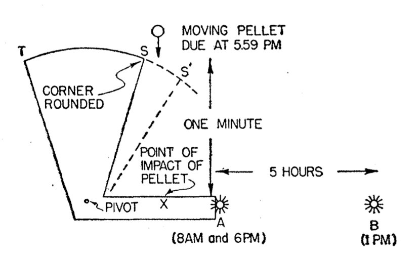
To formulate the paradox acceptably, we have to eliminate human intervention. We therefore introduce a mechanism which saves charge $a$ from a blow at 6 p.m only if this particle performs the expected movement at 8 a.m. (Fig. 1). Our dilemma now is this: Is $a$ hit in the evening or is it not. If it is, then it suffered a premonitory displacement at 8 a.m. which cut off the blow, so $a$ is not struck at 6 p.m.! If it is not bumped at 6 p.m. there is no morning movement to cut off the blow and so in the evening $a$ is jolted!

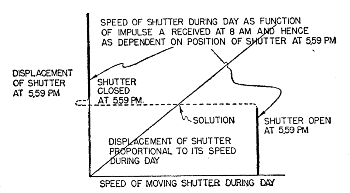
To resolve, we divide the problem into two parts: effect of past of $a$ upon its future, and of future upon past. The two corresponding curves in Fig. 2 do not cross. We have no solution, because the action of the shutter on the pellet, of the future on the past, has been assumed discontinuous in character.

While this paper does not deal directly with general relativity, it was an inspiration for further examples dealing with closed timelike curves, such as Clarke's paper "Time in general relativity" :

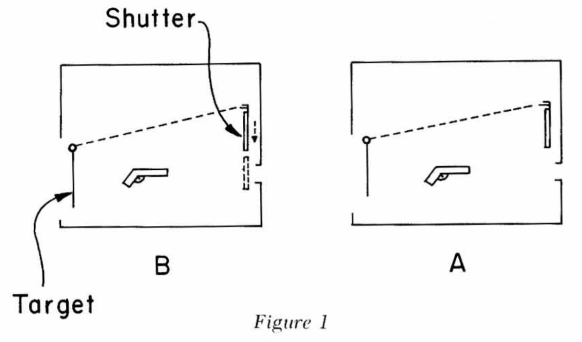
To see how this is so, consider the case already cited of a person who meets his former self in circumstances in which, if physics were normal, he would be able to shoot him. Then, as a preliminary step in the analysis, let us replace the complex human being by a simple automaton which nonetheless exhibits the abnormal physics referred to. This apparatus is to consist of a gun, a target, and a shutter so arranged that the impact of a bullet on the target will trigger the shutter so as to move in front of the gun. It pursues a causality-violating curve in spacetime in such a way that two points on the object's world line $A$ and $B$, with $B$ later in the object's history than $A$, are physically contemporaneous and disposed as in Figure 1 so that the gun at $B$ is aimed at the target at $A$ and the shutter is initially up at $A$.

Suppose now that the machine "shoots its former self" : the gun at $B$ is fired, either by an automatic timing mechanism or by the intervention of a human being making a conscious decision. If the shutter in $B$ were still up, the bullet would strike the target at $A$, which would cause the shutter in $B$ to be down, a contradiction. But if the shutter were down in $B$, then the bullet would be stopped, the target $A$ would not be hit, and the shutter in $B$ should still be up: the shutter is up if, and only if, it is down; the situation is logically impossible.

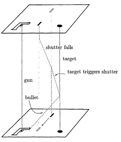
The though experiment is later found in Kriele's "Spacetime : Foundations of general relativity and differential geometry" :

At a first glance, the possibility of "free will" seems to be at the center of the issue. However, following (Wheeler and Feynman 1949) Clarke (1977) has re-formulated the thought experiment in terms of a simple machine and has argued that the thought experiment is fallacious : Assume that there is a gun directed at a target in spacetime. This target is connected with a shutter which, if closed, blocks off the path between the gun and the target : If the gun is triggered, the bullet will hit the target which in turn will cause the shutter to fall. A second shot will now be blocked by the shutter and therefore cannot hit the target (c.f. Fig. 8.1.3). Now assume that the configuration is located in a region with causality violation such that the shutter falls along a closed timelike curve so that it blocks the bullet before the gun has been triggered. Again we seem to arrive at a contradiction : If the shutter is open the bullet can hit the target. But the target closes the shutter which in turn blocks the path of the bullet.

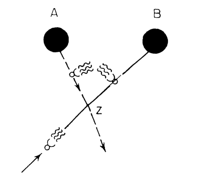
A slightly more radical version of this paradox was made in Novikov's paper "Time machine and self-consistent evolution in problems with self-interaction", in which a ball containing a bomb (exploding upon contact) is sent through a wormhole.

The initial data are arranged in such a way that the ball enters mouth $B$, emerges from mouth $A$ in the past, continues the motion and arrives at the point $Z$ just in time to collide with the "younger" version itself. This encounter leads to the explosion. We did not take into account the influence of the future on the past before the ball entered the mouth $B$, and this is the reason for the "paradox."

But there is a self-consistent evolution, as shown in Fig. 6. The initial data are the same as in Fig. 5, but before reaching the point Z it meets the fragment of the explosion of itself. This fragment hits the ball and it is the cause of the explosion, the fragments of the ball fly in all directions with velocities much larger than the velocity of the ball. Some of them fly into mouth Band emerge from mouth $A$ in the past. One can show that they will continue to fly in practically all directions from mouth A, because they have different impact parameters when they few into mouth $B$. One of the fragments from mouth $A$ crosses the trajectory of the ball at the point $Z'$ exactly at that moment when the ball arrives at the same point $Z'$. This fragment is the cause of the explosion of the ball. The consequence of the explosion (the fragment) is the cause of the explosion.

A variation on this experiment follows as

Now let us consider the problem which is a more complicated version of the problem of the preceding section. The problem is the following (see Figs. 7—9). Let us suppose that there is the ball with a bomb and a radio transmitter (see Fig. 7), which gives a directed beam. The fuse explodes the bomb if, and only if, it is irradiated by the beam of such a radio transmitter from a distance of, say, $30\ m$ (see Fig. 7).

The self-inconsistent evolution is shown in Fig. 8. The "younger" ball explodes, on being irradiated by the radio transmitter of the "older" ball after it comes from the future.

Now a fragment of the explosion cannot be the cause of the explosion and at first glance, the problem of constructing a self-consistent evolution looks insoluble, but that is not the case.

In Fig. 9 one can see the self-consistent evolution. Before reaching the mouth $B$ the "younger" ball encounters its "older" self from the future but with a change orientation of the radio transmitter (in fact the "younger" ball with the radio transmitter rotates after the point $Z$, and the "older" one rotates also). Now the fuse is not irradiated by the radio transmitter and there is no reason for the explosion. The inelastic collision of the "older" and the "younger" versions of the ball leads to a change in the orientation of the radio transmitters of both balls (rotation of the balls ) and drives both of them into slightly altered trajectories. Self-consistent evolution without an explosion is possible.

There are many such occurences of the grandfather paradox here and there in the literature, but those are some of the most famous instances. Some more cases can be found for instance in Earman's "Bangs, Crunches, Whimpers and Shrieks".

Beyond thought experiments, they also do pop up in proposals of actual experiments. Eric Davies, while investigating the Bertotti-Robinson spacetime in his paper "Interstellar Travel Through Magnetic Wormholes" (or as they reference it, the Levi-Civitta spacetime), which was suspected to be a wormhole-like solution by Claudio Maccone (this was later shown to be incorrect). As the Bertotti-Robinson spacetime corresponds to a homogeneous electric or magnetic field, the experimental proposal for the largest effect was to use a nuclear weapon to produce the largest possible magnetic field.

It will be necessary to consider advancing the state-of-art of magnetic induction technologies in order to reach static field strengths that are $> 10^9 - 10^{10}$ Tesla. Extremely sensitive measurements of $c$ at the one part in $10^6$ or $10^7$ level may be necessary for laboratory experiments involving field strengths of $\approx 10^9$ Tesla. Magnetic induction technologies based on nuclear explosives/implosives may need to be seriously considered in order to achieve large magnitude results. An order of magnitude calculation indicates that magnetic fields generated by nuclear pulsed energy methods could be magnified to (brief) static values of $\approx 10^9$ Tesla by factors of the nuclear-to-chemical binding energy ratio ($\approx 10^6$).

Index notation, where a summation over some set is indicated by subscripts and superscripts, can be a curse in physics, as things can go crazy pretty fast for some systems. This usually occurs either when the equations require a large amount of them due to the sheer number of terms or just their variety, in the case of the most esoteric physics.

For instance, he's an example from my own master thesis, where some calculation required me to compute Taylor terms up to the 4th order :

\begin{align} \psi (x_2,t + \epsilon ) &=\sqrt{\frac{m}{2\hbar\pi i\varepsilon}} \int_{-\infty}^{\infty} d\eta\ e^{\frac{im}{2\hbar} g_{ab}(x_2) \frac{\eta^a\eta^b}{\varepsilon}}\nonumber\\ &(1 - \frac{im}{2\hbar\varepsilon}(\lambda \eta^\mu \eta^\nu \eta^\rho g_{\mu\nu,\rho})- \frac{m^2}{8\hbar^2\varepsilon^2}(\lambda^2 \eta^\mu \eta^\nu \eta^\rho \eta^\sigma ( g_{\mu\nu,\rho\sigma}+ \eta^\tau \eta^\chi g_{\sigma\tau,\chi}g_{\mu\nu,\rho})) +\mathcal{O}(\eta^7))\nonumber\\ &(1 +\frac{im}{2\hbar\epsilon} g_{ab}(\tilde{x}) C^{ab}- \frac{m^2}{8\hbar^2\epsilon^2} g_{ab}(\tilde{x})g_{pq}(\tilde{x})C^{ab}C^{pq}+\mathcal{O}(C^3)) \nonumber\\ &(\psi(x_2,t)+ \eta^\alpha \psi(x_2,t)_{,\alpha}+ \frac 12 \eta^\alpha \eta^\beta \psi(x_2,t)_{,\alpha\beta} +\mathcal{O}(\eta^3)) \nonumber\\ &(\sqrt{g(x_2)} + \eta^\aleph \sqrt{g(x_2)}_{,\aleph}+ \frac 12 \eta^\aleph \eta^\beth \sqrt{g(x_2)}_{,\aleph\beth}+ \mathcal{O}(\eta^3)) \end{align}

with some hebrew letters added for fun. Index notation is a topic of some humor, for instance from this parody paper :

We use the following notation: Greek letters for vile spinor indices, Roman letters for isospin indices, Cyrillic letters for vector indices, Hebrew letters for 10-dimensional vector indices, Roman numerals for Dirac spinor indices, and radiation therapy for Hodgkin's disease.

Due to this, indexes tend to be dropped, assumed to be implicit by the choice of objects used in the equation. This happens a lot for spinors, in particular.

Let's now see what we could do with the opposite approach, to use as many indexes as possible. Take for example the Dirac equation, in pure unindexed form :

$$(i\hbar \partial\!\!\!/ - mc) \psi = 0$$

The Feynman slash notation $\partial\!\!\!/$ implies here a summation over two spacetime indexes with Dirac's gamma matrices, $\gamma^\mu \partial_\mu$ (this isn't strictly speaking two spacetime indexes since $\gamma$ isn't a tensor but a soldering form, but it is close enough to it). The equation then becomes

$$(i\hbar \gamma^\mu \partial_\mu - mc) \psi = 0$$

For a total of a single index. From there, we'll have to add the actual spinor indices. There are four types of spinor indices, all noted with upper case letters : the basic spinor $\psi^A$, the dual space spinor $\psi_A$, the complex conjugate spinor $\psi^{\dot A}$ and the complex conjugate dual spinor $\psi_{\dot A}$. The spinor of the Dirac equation is actually none of those, but a vector of spinors called the Dirac bispinor.

$$\psi = \begin{pmatrix}\xi^{A}\\\chi^{\dot A}\end{pmatrix}$$

$\xi$ is the left-handed spinor while $\chi$ is the right-handed spinor. In that notation, the gamma matrices become a matrix of the solder forms on those spinors.

$$\gamma^\mu = \begin{pmatrix} 0 && \sigma^\mu_{A\dot A}\\ \bar \sigma^\mu_{A\dot A} && 0 \end{pmatrix}$$

This allows for instance the usual formula to map a spinor to a vector via $\psi^{\dot A} \sigma^\mu_{A\dot A} \psi^A$. The Dirac equation then becomes

\begin{eqnarray} i\hbar (\sigma^\mu_{A\dot A} \partial_\mu - mc I_{A\dot A})\chi^A &=& 0\\ i\hbar (\bar \sigma^\mu_{A\dot A} \partial_\mu - mc I_{A\dot A}) \xi^A &=& 0 \end{eqnarray}

$I$ simply being the identity matrix. We can set the mass to $0$ and end up with the Weyl equation for a single right-handed spinor with no loss of indexes.

$$i\hbar (\sigma^\mu_{A\dot A} \partial_\mu - mc I_{A\dot A})\chi^A = 0$$

Up to three indexes. Now we go onto gauge fields : we replace the partial derivative $\partial_\mu$ with the gauge derivative $\nabla_\mu$. Gauge derivatives are Kozsul connection on a principal bundle and as such are fairly complicated, something of the form (up to some physical factors)

$$\nabla_\mu = \partial_\mu + \tau_\alpha^{ij} A_\mu^\alpha$$

Where $A$ is the gauge field and $\tau$ is the representation of the gauge group. In our case, we'll want to see the gauge derivative of a product of gauge groups, such as $\mathrm{SU}(3) \times \mathrm{SU}(2) \times \mathrm{U}(1)$, for which it will be a sum of the form

$$\nabla_\mu = \mathrm{I}^{ij} \mathrm{I}^{kl} \mathrm{I}^{mn} \partial_\mu + \tau_\alpha^{ij} G_\mu^\alpha \mathrm{I}^{kl} \mathrm{I}^{mn} + \mathrm{I}^{ij} \sigma_\alpha^{kl} W_\mu^\alpha \mathrm{I}^{mn} + \mathrm{I}^{ij} \mathrm{I}^{kl} u^{mn}_\alpha B_\mu^\alpha $$

$G$ is the gluon field, with $\tau$ the Gell-Mann matrices, $W$ is the weak isospin field, with $\sigma$ the Pauli matrices, and $B$ is the weak hypercharge field, with $u$ simply being some one dimensional matrix (we could remove its indices but let's keep it). The spinor field itself is a product of the original spinor space $\mathbb C^2$, $\chi^A_{ikm}$, each index corresponding to a different charge of the standard model. If we drop the mass term (to avoid getting too long), the new equation then becomes something like

$$i\hbar (\sigma^\mu_{A\dot A} (\mathrm{I}^{ij} \mathrm{I}^{kl} \mathrm{I}^{mn} \partial_\mu + \tau_\alpha^{ij} G_\mu^\alpha \mathrm{I}^{kl} \mathrm{I}^{mn} + \mathrm{I}^{ij} \sigma_\alpha^{kl} W_\mu^\alpha \mathrm{I}^{mn} + \mathrm{I}^{ij} \mathrm{I}^{kl} u^{mn}_\alpha B_\mu^\alpha) ) \chi^A_{ikm} = 0$$

Although we could have arbitrarily many indexes here, for a reasonable theory we are up to 10. We can then add the various flavors of particles. Considering every particle as a variation of the triplet, doublet and singlet of the standard model, there are six of them : the three couples of leptons and their neutrinos $(e, \nu_e)$, $(\mu, \nu_\mu)$ and $(\tau, \nu_\tau)$, and the three generations of quarks, $(u,d)$, $(c,s)$ and $(b,t)$. Without the mass term, we can simply add the flavor index (otherwise, the mass term would depend on both the flavor and the charges)

$$i\hbar (\sigma^\mu_{A\dot A} (\mathrm{I}^{ij} \mathrm{I}^{kl} \mathrm{I}^{mn} \partial_\mu + \tau_\alpha^{ij} G_\mu^\alpha \mathrm{I}^{kl} \mathrm{I}^{mn} + \mathrm{I}^{ij} \sigma_\alpha^{kl} W_\mu^\alpha \mathrm{I}^{mn} + \mathrm{I}^{ij} \mathrm{I}^{kl} u^{mn}_\alpha B_\mu^\alpha) ) \chi^A_{ikmf} = 0$$

Now we can add curved spacetime to the mix. This changes two things : we replace spacetime indices with frame indices (and add the frame field), and we also need another connection, this time the $\mathrm{SO}(1,3)$ connection of the frame bundle.

$$i\hbar (e^\mu_a \sigma^a_{A\dot A} (\mathrm{I}^{ij} \mathrm{I}^{kl} \mathrm{I}^{mn} \partial_\mu + \tau_\alpha^{ij} G_\mu^\alpha \mathrm{I}^{kl} \mathrm{I}^{mn} + \mathrm{I}^{ij} \sigma_\alpha^{kl} W_\mu^\alpha \mathrm{I}^{mn} + \mathrm{I}^{ij} \mathrm{I}^{kl} u^{mn}_\alpha B_\mu^\alpha) + \sigma^a_{A\dot A} \omega_\mu^\alpha S_{\alpha A}) \chi^A_{ikmf} = 0$$ [...]

While rarely done, it is entirely possible to write quantum states in index notation, since they are vectors themselves. For instance, take the two wavefunctions $\Psi$ and $\Phi$. We can write their product as

$$\langle \Psi, \Phi \rangle = \Psi_{\alpha} \Phi^\alpha$$

We can then add the wavefunction to the equation of motion via the Schwinger-Dyson equation

$$\left\langle \frac{\delta S}{\delta \phi(x)} \right\rangle = \Psi_\alpha \left(\frac{\delta S}{\delta \phi(x)}\right)^\alpha_\beta \Psi^\beta = 0$$

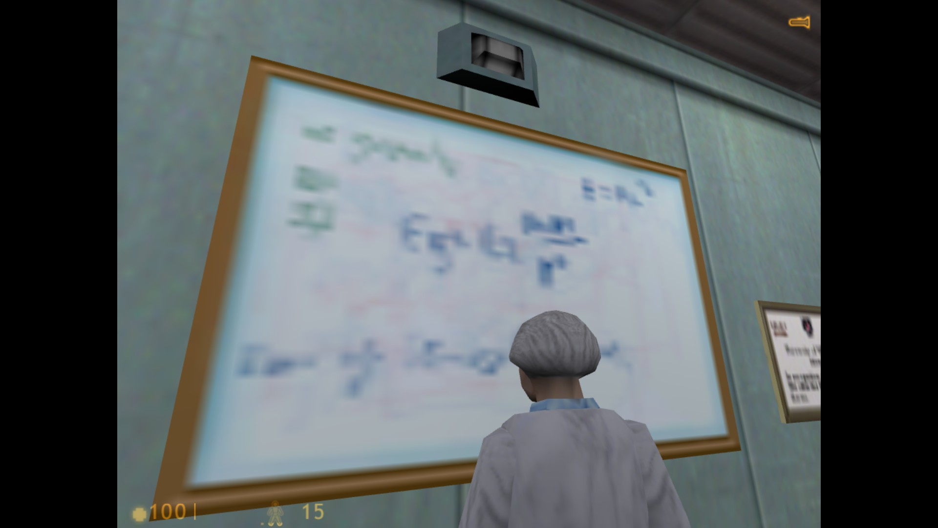
The original Half-Life had rather low resolution whiteboards, making it difficult to fit much legible text on it. All the whiteboards at Black Mesa were the same texture

With the same formulas, which were mostly easily recognizable equations, such as $E = mc^2$ and the Newtonian gravity

$$F_g = G\frac{Mm}{r^2}$$

For the fanmade recreation of Half-Life 1 in the Source engine, Black Mesa, the whiteboards were spruced up by making them higher resolution, with relevant content and unique for each room, although still fairly unrealistic in how well-written and small the text is on a laboratory whiteboard. A good compilation of all the whiteboards is available here. I'll look into the content of the theoretical physics-related ones, as I'm not particularly good with chemistry, crystallography or alien biology.

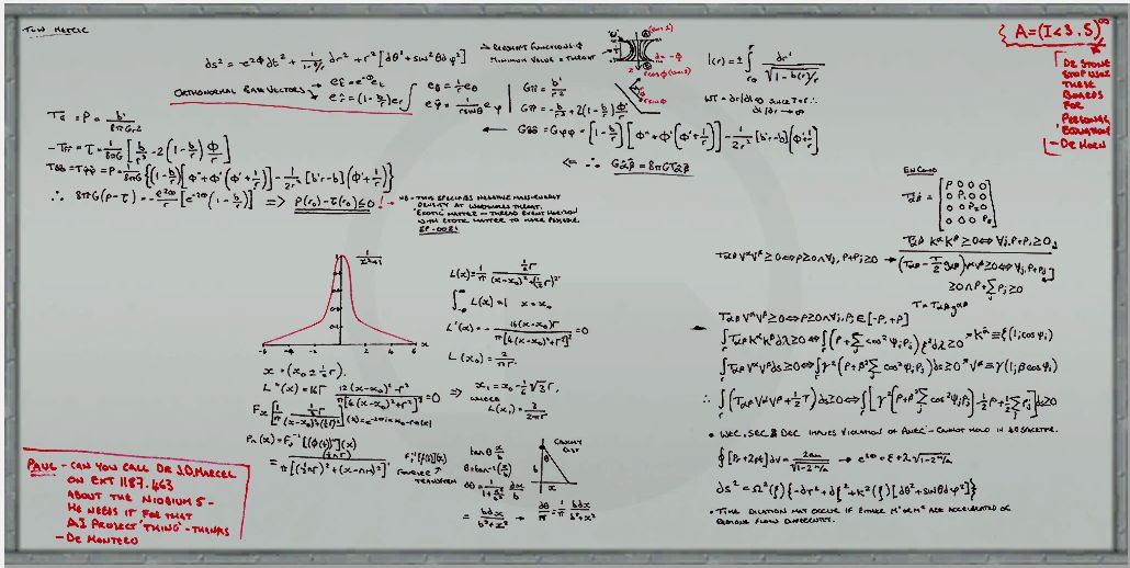
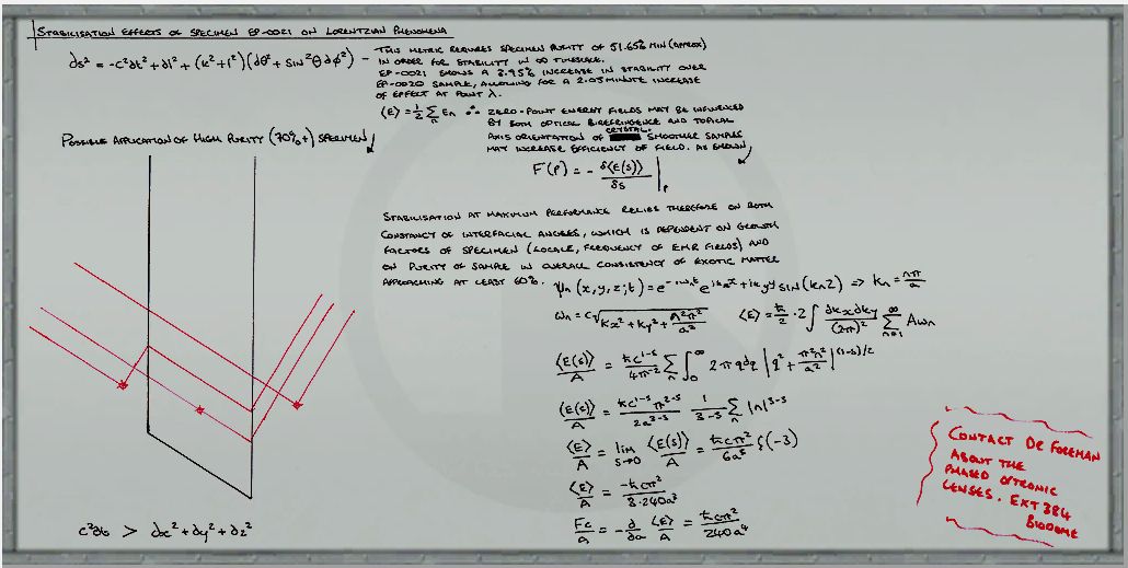
The first few whiteboards are about wormholes and faster-than-light travel, as befits Black Mesa's research on teleportation (although they appear in Sector C, which is more material science, not in Sector F, the Lambda Complex, where the actual teleportation research happens). The first one is on wormholes :

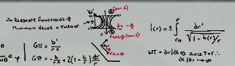
Let's break this down a bit. The first important line is this

$$ds^2 = -e^{2\Phi} dt^2 + \frac{1}{1 + \frac{b}{r}} dr^2 + r^2 \left[ d\theta^2 + \sin^2 \theta d\varphi^2 \right]$$

This is the metric tensor of the Morris-Thorne wormhole, expressed in the Schwarzdchild coordinates. From then on, the rest of the whiteboard roughly follows the same procedure as Morris and Thorne's original paper, Wormholes in spacetime and their use for interstellar travel: A tool for teaching general relativity. To the right are the properties of the functions making up the metric tensor.

Defining $\Phi$ as the redshift function, and putting the throat of the wormhole as the minimum value [of the shape function $b(r)$]. A drawing of the embedding of the surface defined by $(t= \text{const}, r, \theta = \pi/2, \varphi)$ is done, embedded in the three-dimensional space with cylindrical coordinates $(r, \varphi, z)$.

The proper radial distance $l$ is then defined with

$$l(r) = \pm \int_{r_0}^r \frac{dr'}{\sqrt{1 - \frac{b(r)}{r}}}$$

It's a bit hard to make out exactly what they ask but from context it seems to be the usual requirement that $dr/dl = 0$ at the throat, or equivalently $dl/dr \to \infty$ [this implies that at the throat ($r = r_0$), we have $b(r_0) = r_0$].

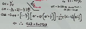
Once the metric is dealt with, they define a tetrad (a set of orthonormal basis vectors)

\begin{eqnarray} e_{\hat{t}} &=& e^{-\Phi} e_t\\ e_{\hat{r}} &=& (1 - \frac{b}{r}) e_r\\ e_{\hat{\theta}} &=& \frac{1}{r} e_\theta\\ e_{\hat{\varphi}} &=& \frac{1}{r\sin \theta} e_\varphi \end{eqnarray}

Then they compute the Einstein tensor along that tetrad

\begin{eqnarray} G_{\hat{t}\hat{t}} &=& \frac{b'}{r^2}\\ G_{\hat{r}\hat{r}} &=& - \frac{b}{r^3} + 2 (1 - \frac{b}{r}) \frac{\Phi'}{r}\\ G_{\hat{\theta}\hat{\theta}} &=& G_{\hat{\varphi}\hat{\varphi}} = \left[ 1 - \frac{b}{r} \right] \left[ \Phi'' + \Phi' (\Phi' + \frac{1}{r}) \right] - \frac{1}{2 r^2} \left[ b'r - b\right] \left[ \Phi' + \frac{1}{r} \right] \end{eqnarray}

And from there, using the Einstein field equations $G_{\hat{\alpha}\hat{\beta}} = 8\pi G T_{\hat{\alpha}\hat{\beta}}$, they compute the stress-energy tensor, and associated to it, the energy density $\rho$, the radial tension $\tau$ and the tangential pressure $p$.

\begin{eqnarray} T_{\hat{t}\hat{t}} &=& \rho = \frac{b'}{8 \pi G r^2}\\ - T_{\hat{r}\hat{r}} &=& \tau =\frac{1}{8 \pi G} \left[ - \frac{b}{r^3} + 2 (1 - \frac{b}{r}) \frac{\Phi'}{r}\right]\\ T_{\hat{\theta}\hat{\theta}} &=& T_{\hat{\varphi}\hat{\varphi}} = p = \frac{1}{8\pi G} \left\{ \left[ 1 - \frac{b}{r} \right] \left[ \Phi'' + \Phi' (\Phi' + \frac{1}{r}) \right] - \frac{1}{2 r^2} \left[ b'r - b\right] \left[ \Phi' + \frac{1}{r} \right] \right \} \end{eqnarray}

They then compute the quantity $\rho - \tau$, which is the product of the stress-energy tensor with a null curve of tangent $k^{\hat{\mu}} = (1, 1, 0, 0)$ in the tetrad basis, that is

$$T_{\hat{\alpha}\hat{\beta}} k^{\hat{\alpha}} k^{\hat{\beta}} = \rho - \tau$$

$ 8 \pi G(\rho - \tau)$ corresponding to the Einstein tensor $G_{\hat{\alpha}\hat{\beta}} k^{\hat{\alpha}} k^{\hat{\beta}}$. This quantity is then found to be equal to

$$ 8 \pi G(\rho - \tau) = - \frac{e^{2\Phi}}{r} \left[ e^{-2\Phi} (1 - \frac{b}{r}) \right]' $$

Since $b(r)$ has a minima at the throat of the wormhole ($r = r_0$) where $b(r_0) = r_0$, and any point beyond the throat will have $b(r) < r$, this leads to

$$e^{-2\Phi} (1 - \frac{b}{r}) > 0$$

Meaning that there is at least one point superior to $r_0$ where the derivative is positive, in particular this will be true at the throat itself, hence

$$ 8 \pi G(\rho(r_0) - \tau(r_0)) \leq 0$$

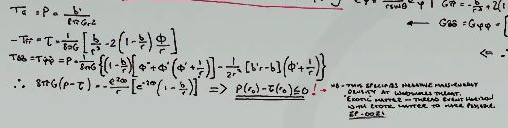
which means that the throat requires exotic matter, as the comment indicates. The details of why this is so is in the following section

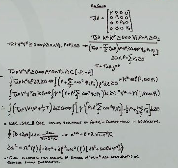
This starts first with writing the stress-energy tensor in matrix form. Since the metric leads to a Type I stress energy tensor, it is of the form

$$T_{\hat{\alpha}\hat{\beta}} = \begin{bmatrix} \rho &0&0&0 \\ 0 & p_1 & 0 & 0 \\ 0 & 0 & p_2 & 0 \\ 0 & 0 & 0 & p_3 \end{bmatrix}$$

Then the Null Energy Condition (or NEC) is written down. The NEC states that given any null vector, the product of the stress-energy tensor with those vectors is positive or null,

$$T_{\alpha \beta} k^{\alpha} k^{\beta} \geq 0$$

For Type I stress-energy tensors, this will correspond to the following condition

$$\forall j, \rho + p_j \geq 0$$

that is, the sum of the energy density and momentum density in any direction is positive or zero, which is precisely the condition violated by the metric, for the radial momentum. The next equations concern other energy conditions, starting with the Weak Energy Condition (or WEC), which states that for any timelike vector $V$, we have

$$T_{\alpha \beta} V^{\alpha} V^{\beta} \geq 0$$

meaning that, for a Type 1 stress-energy tensor, we get

$$\rho \geq 0 \wedge \forall j, \rho + p_j \geq 0$$

The energy density is positive or zero, as well as its sum with the momentum density in any direction, which is also rewritten as $p_i \in [-\rho, \rho]$ later.

Then there is the Strong Energy Condition (or SEC)

$$(T_{\alpha \beta} + \frac{T}{2} g_{\alpha \beta}) V^{\alpha} V^{\beta} \geq 0$$

with $T = T_{\alpha \beta} g^{\alpha \beta}$, which can once again be rewritten as

$$\forall j, \rho + p_j \geq 0 \wedge \rho + \sum_j p_j \geq 0$$

The next three lines are the averaged versions of those energy conditions, the averaged null energy condition (ANEC), averaged weak energy condition (AWEC) and averaged strong energy condition (ASEC). For any curve $\gamma$ with tangent vector $k$ or $V$,

\begin{eqnarray} \int T_{\alpha \beta} k^\alpha k^\beta d\lambda &\geq& 0\\ \int T_{\alpha \beta} V^\alpha V^\beta d\tau &\geq& 0\\ \int (T_{\alpha \beta} k^\alpha k^\beta + \frac{1}{2} T) d\tau&\geq& 0 \end{eqnarray}

For a tangent vector $k^\alpha = \xi (1; \cos \psi_i)$ and $V^\alpha = \gamma (1; \beta \cos \varphi_i)$, this gives the relations \begin{eqnarray} \int (\rho + \sum_j \cos^2 \psi_j p_j) \xi^2 d\lambda &\geq& 0\\ \int (\rho + \beta^2 \sum_j \cos^2 \varphi_j p_j) \gamma^2 &\geq& 0\\ \int \left[ \gamma^2 (\rho + \beta^2 \sum_j \cos^2 \varphi_j p_j) \frac{1}{2} \rho + \frac{1}{2} \sum_j p_j \right] d\tau&\geq& 0 \end{eqnarray}

The follow-up isn't too clear, outside of the bit of text saying that violation of the WEC, SEC and DEC implies a violation of the ANEC (which is true).

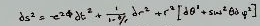
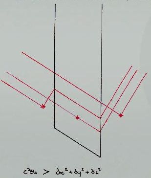
Another whiteboard contains a few different things concerning faster-than-light travel.

First there is this metric tensor

$$ds^2 = -c^2 dt^2 + dl^2 + (k^2 + l^2) (d\theta^2 + \sin^2 \theta d\varphi^2)$$

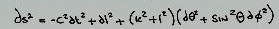
This is actually the same metric as previously, except that it is in the proper distance coordinate system, using the relation $l(r)$ seen above, giving the metric $$ds^2 = -c^2 dt^2 + dl^2 + r^2(l) (d\theta^2 + \sin^2 \theta d\varphi^2)$$

with the radius function $r = \sqrt{l^2 + k^2}$, corresponding to the Ellis-Bronnikov wormhole.

The diagram

isn't actually the corresponding spacetime, but it is the diagram of the Kranikov tube, showing the light cones at various points, $c^2 dt^2 > dx^2 + dy^2 + dz^2$ simply indicating timelike curves.

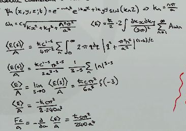
The final part of the whiteboard concerns the Casimir effect

While realistically not ideal for propping up wormholes or Krasnikov tubes, the Casimir effect is a simple example of violation of most energy conditions, which wormholes do require. It's a fairly standard treatment (once again seemingly taken from the wikipedia article on the topic), first defining the eigenfunctions of a scalar field between two conducting plates separated by a length $a$ along the $z$ axis

$$\psi_n(x,y,z;t) = e^{-i\omega_n t} e^{ik_x x + i k_y y} \sin(k_n z)$$

with the momentum in the $z$ direction quantized as $k_n = \pi n / a$, and correspondingly the dispersion relation for the frequency

$$\omega_n = c \sqrt{k_x^2 + k_y^2 + \frac{\pi^2 n^2}{a^2}}$$

The expectation value of the energy of that field being

$$\langle E \rangle = \frac{\hbar}{2} 2 \int \frac{dk_x dk_y}{(2\pi)^2} \sum_{i= 1}^\infty A \omega_n$$

If we define $q^2 = k_x^2 + k_y^2$ and switch to polar coordinates, the integral becomes

$$\langle E \rangle = \frac{\hbar}{2} 2 \int \frac{1}{(2\pi)} r dr \sum_{i= 1}^\infty A \omega_n$$

or

$$\langle E \rangle = \frac{\hbar}{2} 2 \int \frac{1}{(2\pi)} r dr \sum_{i= 1}^\infty A c \sqrt{q^2 + \frac{\pi^2 n^2}{a^2}}$$

This quantity is fairly divergent, just being an integral of an unbounded positive function over $\mathbb R$, as well as an infinite sum of a strictly increasing function, so we need to perform a regularization, in this case with the use of a zeta regulator. Instead of summing the quantity $\omega_n$, we'll sum $\omega_n |\omega_n|^{-s}$, with the limit $s \to 0$. This gives the appropriate forumla

$$\frac{\langle E(s) \rangle}{A} = \frac{\hbar c^{1 - s}}{4\pi^{2}} \sum_n \int_0^\infty 2\pi q dq |q^2 + \frac{\pi^2 n^2}{a^2}|^{\frac{1-s}{2}} $$

with the integral evaluating to

$$\frac{\langle E(s) \rangle}{A} = - \frac{\hbar c^{1 - s} \pi^{2 - s}}{2 a^{3-s}} \frac{1}{3-s} \sum_n |n|^{3-s}$$

Which is obviously divergent for $s = 0$. This corresponds to the limit of $s \to 0$ of the Riemann zeta function $\zeta(s - 3)$. While the Riemann zeta function isn't well-defined around that point, it is possible to analytically continue it in that region. We can then obtain

$$\frac{\langle E \rangle}{A} = \lim_{s \to 0} \frac{\langle E(s) \rangle}{A} = - \frac{\hbar c \pi^2}{6 a^3} \zeta(-3)$$

And the analytical continuation of $\zeta$ gives

$$\zeta(-3) = \frac{1}{120}$$

For a total energy of

$$\frac{\langle E \rangle}{A} = -\frac{\hbar c \pi^2}{720 a^3}$$

It is followed by a simple calculation of the Casimir force generated by moving the plates,

$$\frac{F_c}{A} = - \frac{d}{da} \frac{\langle E \rangle}{A} = -\frac{\hbar c \pi^2}{240a^4}$$

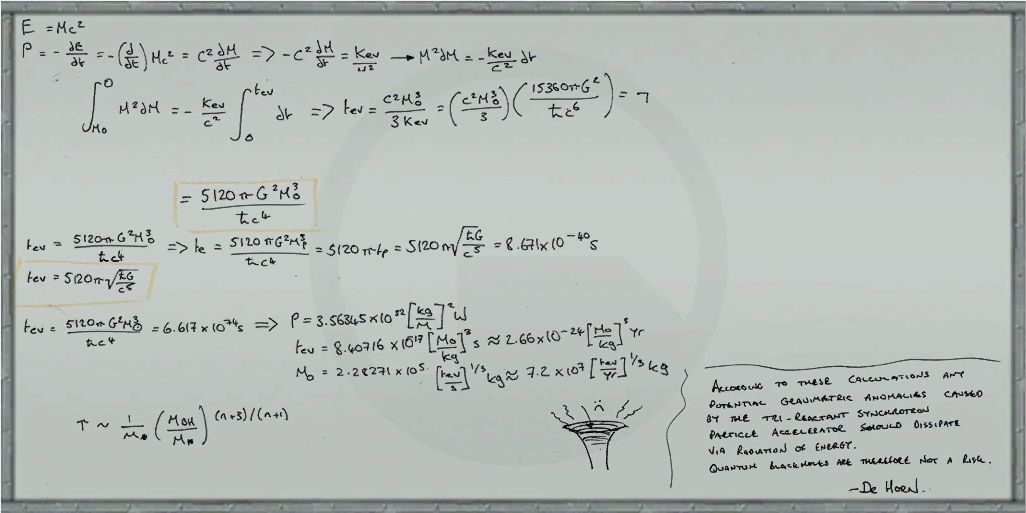
The following whiteboard is a calculation of evaporation time for Schwarzschild black holes via Hawking radiation (the derivation of which is possibly taken from the wikipedia article on the topic) :

Consider a black hole of mass $M$, corresponding to a total energy of $E = Mc^2$. The total power radiated will be equal to the change in its energy

$$P = -\frac{dE}{dt} = -c^2 \frac{dM}{dt}$$

The power radiated $P$ is known from the Hawking derivation of the radiation

$$P = \frac{\hbar c^6}{15360 \pi G^2 M^2}$$

of which we will split out the mass to obtain

$$P = \frac{K_{ev}}{M^2},\ K_{ev} = \frac{\hbar c^6}{15360 \pi G^2}$$

Then we can simply solve the evaporation time as a simple ordinary differential equation of the mass, via

$$-c^2 \frac{dM}{dt} = \frac{K_{ev}}{M^2}$$

meaning that the energy radiated away is lost to the total mass. Using the common physicist trick of treating differentials as real objects, we get

$$M^2 dM= -\frac{K_{ev}}{c^2} dt$$

The black hole starts at time $t = 0$ at mass $M = M_0$ and finishes at time $t = t_{ev}$ at mass $M = 0$, with the solution

$$\int_{M_0}^0 M^2 dM= -\frac{K_{ev}}{c^2} \int_{0}^{t_ev} dt \Rightarrow - \frac{M_0^3}{3} = -\frac{K_{ev}}{c^2} t_{ev}$$

which gives us the evaporation time as

\begin{eqnarray} t_{ev} &=& \frac{c^2 M_0^3}{3 K_{ev}} = (\frac{c^2 M_0^3}{3} ) (\frac{15360 \pi G^2}{\hbar c^6})\\ &=& \frac{5120 \pi G^2 M_0^3}{\hbar c^4} \end{eqnarray}

The rest of the calculations are just the evaporation times for two masses : the Planck mass and one solar mass. For the Planck mass

$$M_P = \sqrt{\frac{\hbar c}{G}}$$

the corresponding evaporation time is

$$t_{ev} = \frac{5120 \pi G^2 M_p^3}{\hbar c^4} = 5120 \pi t_p = 5120 \pi \sqrt{\hbar G}{c^5} \approx 8.671 \times 10^{-40} s$$

while for one solar mass,

$$t_{ev} = \frac{5120 \pi G^2 M_\odot^3}{\hbar c^4} = 6.617 \times 10^{74} s$$

The formulas are then expressed in SI units

$$P = 3.563\,45 \times 10^{32} \left[\frac{\mathrm{kg}}{M}\right]^2 \mathrm{W}$$ $$t_\mathrm{ev} = 8.407\,16 \times 10^{-17} \left[\frac{M_0}{\mathrm{kg}}\right]^3\; \mathrm{s} \quad \approx\ 2.66 \times 10^{-24}\; \left[\frac{M_0}{\mathrm{kg}}\right]^3\; \mathrm{yr}$$ $$M_0 = 2.282\,71 \times 10^5\;\left[\frac{t_\mathrm{ev}}{\mathrm{s}}\right]^\frac13\; \mathrm{kg} \quad \approx\ 7.2 \times 10^7\; \left[\frac{t_\mathrm{ev}}{\mathrm{yr}}\right]^\frac13\; \mathrm{kg}$$

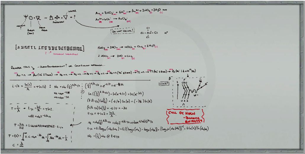
While the first part is some sort of mix of chemical and alchemical notation, the second is related to radioactive decay. The diagram is the Feynman diagram of a beta netative ($\beta^-$) decay, as seen from the perspective of quantum chromodynamics

with a neutron (composed of three quarks $udd$) emitting a $W^-$ boson, via the process $d \to u + W^-$, turning it into a proton ($uud$). The $W^-$ boson then decays into an electron and anti-electronic neutrino, $W^- \to e^- + \bar \nu_e$.

The text itself is a standard derivation of the eponymous half life formula for radioactive decay. First they define the half-life in terms of the decay constant

$$t_{1/2} = \frac{\ln(2)}{\lambda} = \tau \ln(2)$$ $$N_t = N_0 (\frac{1}{2})^{\frac{t}{t_{\frac{1}{2}}}}$$