Flat vs. round earth

The idea that the Earth is flat is, as far as we can tell, a pretty ancient one, with Bronze Age cosmologies mentioning it, as well as some philosophers. Thales is usually credited as an example, but as the actual text is somewhat ambiguous, a clear example can be found with Anaximander (c. 610 BCE – c. 546 BCE), according to the Stromata (Στρώματα) :

ὑπάρχειν δέ φησι τῷ μὲν σχήματι τὴν γῆν κυλινδροειδῆ, ἔχειν δὲ τοσοῦτον βάθος ὅσον ἂν εἴη τρίτον πρὸς τὸ πλάτος. φησὶ δὲ τὸ ἐκ τοῦ ἀιδίου γόνιμον θερμοῦ τε καὶ ψυχροῦ κατὰ τὴν γένεσιν τοῦδε τοῦ κόσμου ἀποκριθῆναι καί τινα ἐκ τούτου φλογός σφαῖραν περιφυῆναι τῷ περὶ τὴν γῆν ἀέρι ὡς τῷ δένδρῳ φλοιόν· ἧστινος ἀπορραγείσης καὶ εἴς τινας ἀποκλεισθείσης κύκλους ὑποστῆναι τὸν ἥλιον καὶ τὴν σελήνην καὶ τοὺς ἀστέρας.

He says that the earth is cylindrical in form, and that its depth is as a third part of its breadth. He says that something capable of begetting hot and cold was separated off from the eternal at the origin of this world. From this arose a sphere of flame which grew round the air encircling the earth, as the bark grows round a tree. When this was torn off and enclosed in certain rings, the sun, moon, and stars came into existence.

The intuitiveness of the flat Earth gave it some degree of popularity in the pre-modern era, and it was a fairly common feature of cosmological models

The exact appearance of the idea of a spherical Earth is somewhat controversial, with many philosophers positing the ideas at various points, but it is often attributed to Eratosthenes, who experimentally verified it c. 240 BCE. This idea probably stems from a variety of phenomenon involving long distances, as large scales are often needed to get a sense of Earth's global shape : the appearance of the night sky in different places, projected shadows, the timing of sunsets, changes in seasons, temperatures, etc.

The two models

Spherical Earth

The spherical Earth model holds that the Earth is roughly the shape of a ball, while the flat Earth holds that it is roughly the shape of a disk (so that it will be some kind of thin cylinder). Obviously, neither of these models are true, as any cursory glance will tell us, so we're going to have to deal with some uncertainty.

As a good approximation, we can roughly say that any spot on Earth is within ten kilometers of ground level. Furthermore, the spherical model does not assume a perfect sphere for ground level, but roughly an oblate ellipsoidal shape. The surface of an oblate ellipsoid is defined by the constraint

\begin{equation} \frac{x^2 + y^2}{a^2} + \frac{z^2}{b^2} = 1 \end{equation}

The oblateness means that $b > a$. This means that a point at its furthest from the center is at distance $b$, while the closest point will be at distance $a$. In the case of Earth, we have approximately $a = 6,350\ \mathrm{km}$, and $b = 6,380\ \mathrm{m}$.

In terms of spherical coordinates, given by

\begin{eqnarray} r &=& \sqrt{x^2 + y^2 + z^2}\\ \theta &=& \arccos(\frac{z}{\sqrt{x^2 + y^2 + z^2}})\\ \phi &=& \mathrm{atan} 2(y, x) \end{eqnarray}

with $\mathrm{atan} 2$ the usual arctangent function for spherical coordinates. The constraint corresponds then to the boundary being at a distance of

\begin{equation} R_\oplus(\theta, \phi) = \frac{a^2 b}{\sqrt{a^2b^2 (\cos^2(\theta) + sin^2(\theta) \cos^2(\phi)) + a^4 \sin^2(\theta)\sin^2(\phi)}} \end{equation}

This corresponds to an inverse flattening of $f^{-1} \approx 300$. The flattening parameter for an ellipsoid being given by the normalized difference

\begin{equation} f = \frac{a-b}{a} \end{equation} \begin{equation} \frac{x^2 + y^2}{a^2} + \frac{z^2}{b^2} = 1 \end{equation}

Flat Earth

The standard idea of a flat Earth seems to be some cylinder, of thickness $h$ and radius $R$, up to whatever local topology may occur. Let's consider to round up that our thickness $h$ is only defined up to $\pm10\ \mathrm{km}$.

As a cylinder, we will be using standard cylindrical coordinates $(\rho, \theta, z)$. Our flat Earth will be some kind of cylinder with $\rho < \rho_\oplus$, for some unknown radius $\rho_\oplus$, $\theta \in [0, 2\pi]$, and $z \in [-h, 0]$, with $h$ our unknown thickness of the Earth. It's often considered that the azimuthal equidistant projection (centered on the North pole) is the proper representation of the flat Earth, which means that given the latitude and longitude $\phi, \lambda$, we have the relation

\begin{eqnarray} \rho &=& R (\frac{\pi}{2} - \phi)\\ \theta &=& \lambda \end{eqnarray}

Other models

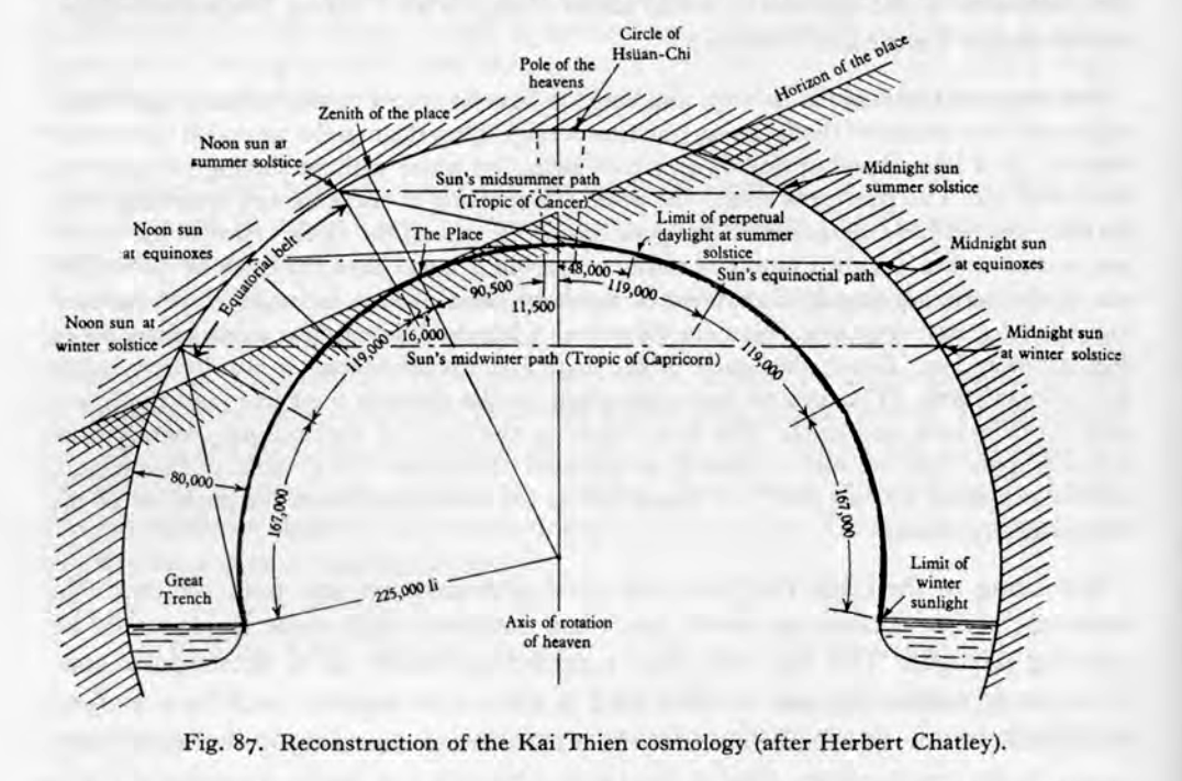
There are of course many models one can choose instead of those two (probably classified by the moduli space of Riemann surfaces), including some intermediate models such as domes that may more closely replicate either model in some characteristics, but these models are rarely considered.

Astronomy

The exact astronomical model isn't quite important here, all we really need is the evolution of the sun's position in the sky. In standard astronomical theory, the position of the sun in the sky is quite complex, so to keep it simple for now let's consider the two following phenomenon :

The Keplerian motion of the Earth around the sun
The rotation of the Earth around its axis

Once this is done, we can change our coordinate system to a point on the surface of the Earth.

The motion of the Earth around the sun in heliocentric coordinates is simple enough, at least as far as the angular formula is concerned. If we consider the sun to be much more massive than the Earth, which it can generally be considered to be, the center of gravity of the system can be considered to be the center of the sun itself (It is about $450km$ off in fact, but this is barely measurable). If we fix the Earth's orbit to be of constant azimuthal angle (which we can do, by the conservation of angular momentum), then the earth will go along an ellipsis

\begin{equation} r(\theta) = \frac{a (1 - e^2)}{1 + e \cos(\theta)} \end{equation}

The horizon

Quite possibly the oldest argument for a spherical Earth is the existence of the horizon, as beyond a given a certain distance, objects are not visible anymore, no matter the elevation one has. The basic idea is quite simple, but there are also some unforeseen complications.

For a spherical Earth, if we consider an observer $A$ at some position $(r_A, \theta_A, \phi_A)$, trying to observe an object $B$ at some position $(r_B, \theta_B, \phi_B)$, we are essentially trying to find if the line connecting $A$ and $B$ intersects with the Earth. As this will depend also on the terrain in between, let's consider the Earth to have a radius $R$, with $R$ the maximal height of the terrain in between $A$ and $B$.

The intersection between a segment $AB$ and a sphere of center $O$ and radius $R$ can be considered as the problem of finding points on the line at a distance from the sphere's center inferior to its radius, or

\begin{equation} \forall x \in AB, d(x, O) \leq R \end{equation}

The set of points between $A$ and $B$ is defined on the line defined by the vector $\vec{B} - \vec{A}$. In this case, the latitude and longitude are not important and we can simply rotate our coordinate system to one where $\phi_A = \phi_B = 0$, and $\theta_A = 0$ without changing the intersection, so that our vector is simply $(r_B - r_A, )$

...

There is no such complication in the flat case, beyond the altitude of the terrain in between, as any observer can see any object if they are both higher than the terrain. If there is no obstacle between two points $(\rho_A, \phi_A, z_A)$ and $(\rho_B, \phi_B, z_B)$ (as long as $z_A, z_B > 0$), there is a clear uninterrupted line.

The complication comes in the case

Optics

A complication of the issues we have looked at previously is that we have only considered geometric arguments, stemming from the properties of straight lines. But actual visual measurements involve the use of light, which does (in the geometric optic limit) go along straight lines.

The path took by light in geometric optic is given locally by Snell's law, where if light moves from one medium to another, its direction changes according to the following law :

\begin{equation} \frac{\sin(\theta_1)}{\sin(\theta_2)} = \frac{n_2}{n_1} = \frac{v_1}{v_2} \end{equation}

where $\theta_1$ and $\theta_2$ are the angles formed by the light ray in the original and new medium and the normal vectors of its incidence point (each vector being directed to go into the medium its describes), and $n_1$, $n_2$ are the refractive indices of the two media, characteristic of the material constituting it. $v_1$ and $v_2$ are the respective phase velocities of light in the two media. It is to be kept in mind that the geometric limit of optics is in the approximation of high frequencies, and this is not actually true in the general case, where waves of different frequencies will be refracted differently, leading to chromatic abberations, but this will not be our focus here.

This formula is best adapted for the interface of two regions of constant refractive indices, but for observations of the type that we consider, this is not the case. The atmosphere's refractive index will vary with temperature, pressure and composition, such as its humidity and carbon dioxide. If we have a continuum of differing refractive indices, we have to use gradient index optics. The usual demonstration is to use Fermat's principle that the path taken by light minimizes travel time, which is then simply the integral

\begin{equation} L = \int_{p}^q n(x,y,z) ds \end{equation}

Gravity

Another fairly important modification to physics if we change the shape of the Earth will be the gravity generated. The gravitational potential is given by

\begin{equation} \Phi(\vec{x}) = - \int \frac{G}{|\vec{x} - \vec{y}|} \rho(\vec{y}) d^3 y \end{equation}

This formula was verified independently of the shape of the Earth, in various experiments such as the Cavendish experiment or the Schiehallion experiment, so that we can use it without worrying too much.

From this formula, we can get the gravitational acceleration of a mass, given by the gradient of the potential

\begin{equation} \vec{a}(\vec{x}) = \vec{\nabla} \Phi(\vec{x}) = - \int \frac{G}{|\vec{x} - \vec{y}|^2} \rho(\vec{y}) d^3 y \end{equation}

This gravitational acceleration has a number of consequences that can be measured experimentally (what is generally called gravimetry). The simplest one being free fall, where an object, neglecting other forces such as friction, will fall under Earth's gravity with the radial acceleration

\begin{equation} \ddot{r}(t) = \vec{a}(\vec{x}) \cdot \vec{e}_r \end{equation}

If we assume that all the matter involved is below the object (so that the shell theorem applies), and that we can assume that the acceleration is constant on the interval we consider (for a fall of $1\ \mathrm{m}$, the change in acceleration is only about $|GM_\oplus / R_\oplus^2 - GM_\oplus / (R_\oplus + \Delta)^2| \approx 3 \times 10^{-6}\ \mathrm{m / s^2}$), then we get the free fall equation

\begin{equation} \ddot{r}(t) = -g \end{equation}

with solution

\begin{equation} r(t) = -\frac{g}{2} t^2 + v_0 t + r_0 \end{equation}

These approximations may not work perfectly in general, since there may be masses nearby above the level of the object (such as mountains), and in the flat case, the amount of mass beyond that radius will depend on the distance from the North Pole, but we will see the exact issue when we get to it.

In the spherical model

Earth's gravity is fairly straightforward in the spherical model, where we simply consider the center of our ellipsoid to be the center of gravity, with a strength that depends on our radius. We can check that, assuming a mass distribution that varies only radially, the center of mass is indeed at the center :

\begin{eqnarray} \vec{C}_\oplus &=& \frac{1}{M_\oplus} \int_\oplus \rho(r) \vec{r} dV \\ &=& \frac{1}{M_\oplus} \int_0^{R_\oplus(\phi, \theta)} \rho(r) r^3 \left[ \int_0^{2\pi} \int_{0}^{\pi} \left( \cos (\theta) \sin (\phi), \sin (\theta) \sin (\phi), \cos (\phi) \right) \sin(\theta) d\theta d\phi \right] dr \\ &=& \frac{1}{M_\oplus} \int_0^{R_\oplus(\phi, \theta)} \rho(r) r^3 \left[ \int_0^{2\pi} \int_{0}^{\pi} \left( \cos (\theta) \sin(\theta) \sin (\phi), \sin^2 (\theta) \sin (\phi), \sin(\theta) \cos (\phi) \right) d\theta d\phi \right] dr \\ &=& \frac{1}{M_\oplus} \int_0^{R_\oplus(\phi, \theta)} \rho(r) r^3 \left[ \int_0^{2\pi} \left( \cos (\theta) \sin(\theta) [-\cos (\phi)]_0^\pi, \sin^2 (\theta) [-\cos(\phi)]_0^\pi, \sin(\theta) [\sin(\phi)]_0^\pi \right) d\theta d\phi \right] \end{eqnarray}

For longitude $\phi$ and latitude $\theta$, ground level in this model will be at a distance of $R_{\oplus}(\theta)$, so that the minimal and maximal gravitational forces will be

\begin{equation} g(\theta) \end{equation}

The standard gravity $g = 9.80665\ \mathrm{m/s^2}$ is generally defined to be the one at (geodetic) sea level at a latitude of $45^\circ$ ($\theta = \pi/4$)

The actual gravitational potential of the Earth can vary quite a bit, depending, in addition of its ellipsoidal shape, on the geology, and even tidal forces from other bodies (mostly the moon), but it is a good first approximation of

In the flat model

In the flat model, the computation of gravity becomes a fair bit more complicated, as we are getting much further from spherical symmetry, although the system remains axially symmetric. If we assume that the mass distribution is axially symmetric, we get

\begin{eqnarray} \vec{C}_\oplus &=& \frac{1}{M_\oplus} \int_\oplus \rho(\rho, z) \vec{r} dV \\ &=& \frac{1}{M_\oplus} \int_{-h}^{0} \int_{0}^{\rho_\oplus} \rho(\rho, z) \rho^2 \left[ \int_0^{2\pi} \left( \rho \cos(\theta), \rho \sin(\theta), z \right) d\theta \right] dr \\ &=& \end{eqnarray}

The center of mass is located at the North Pole, but we cannot guess its depth without additional data. If we assume cylindrical symmetry, it will be at the $-h/2$, but that is about all we can say.

If we do not have data on the mass density of Earth in the flat model, it is difficult to pronounce any number, but we can do some estimations later on. For now, let's fix this depth at some value $h_c \in (0, h)$ and see what we can infer from it.

The distance from this point is the distance from a point along the axis of a cylinder to its boundary disks. given a point on Earth's surface $(\rho, \theta, 0)$, its distance from the center of mass $(0, 0, -h_c)$ can be determined by the Pythagorean theorem with

\begin{equation} r = \sqrt{h_c^2 + \rho^2} \end{equation}

We therefore have two bounds on the gravitational force of flat Earth, given by its value at the North and the South Pole. As we do not have a well-determined radius with which to determine the South Pole's distance, we can also pick another point of well-determined distance.

At the North Pole, the gravitational potential is simply

\begin{equation} \Phi(0, 0, 0) = - \frac{GM_\oplus}{h_c} \end{equation}

Geophysics

A fairly important consequence of the shape of the Earth is its geophysics. The theoretical reason behind the shape of the Earth is that this approximately spherical shape allows it to be near hydrostatic equilibrium, where its gravitational force is balanced by its internal pressure.

Flatness is not inherently forbidden by such problems, as there does exist flat objects in the solar system, such as the comet A/2017 U1 (or ʻOumuamua), which has an aspect ratio (ratio of its longest and shortest axis) estimated between $5$ and $10$. But it will put some constraints on objects over a certain mass and length.

Unlike previous issues, this is fairly complicated and will generally involve the internal composition of Earth, but no matter the internal composition, there is a limit to any material beyond which it will stop being rigid and will start to deform, in some regime such as elastic, plastic or fracture.

Hydrostatic equilibrium

First let's see what hydrostatic equilibrium exactly is. If we can in some limit assume that our planet acts like a fluid (we will see later on how well-founded this approximation is), the planet is in hydrostatic equilibrium if its self-gravity is in equilibrium with its internal pressure at all points of the planet, so that it is static, ie does not move.

Let's consider a basic fluid. A general fluid can be described by the Navier-Stokes equation :

\begin{equation} \rho \frac{D \vec{u}}{Dt} = - \vec{\nabla} p + \vec{\nabla} \cdot \vec{\tau} + \rho \vec{g} \end{equation}

where $\rho$ is the mass density distribution of the fluid, $\vec{u}$ is the flow velocity, $p$ the pressure distribution, $\vec{\tau}$ the viscosity (the deviatoric stress), and $\vec{g}$ a force acting on the fluid (here gravity).

In the hydrostatic limit, we have no flow (the fluid is at rest) : $\vec{u} = 0$, and our quantities are time independent.

\begin{equation} \vec{\nabla} \cdot \vec{\tau} + \rho \vec{g} = \vec{\nabla} p \end{equation}

The potato radius

Actual planets (and objects in general) are however not fluids nor even plastic materials. They are aggregates of rocks and fluids of various properties, and their behaviours under stress can be to move, deform (elastically or plastically) or rupture. A full description of how such bodies actually behave is practically impossible, but there are some simplified models we can use, as well as examples we can look at.

A very rough model is to look at the binding energy of the constitutive materials. The bonds between two atoms or molecules in a solid is roughly between 1 and 10 eV.

Bibliography

A. Jenkins, The Sun's position in the sky, 2013
C. H. Lineweaver, M. Norman, The Potato Radius: a Lower Minimum Size for Dwarf Planets, 2010
B. Edlén, The Refractive Index of Air, 1966

Last updated : 2023-05-08 12:50:20

Tags : physics , astronomy

Bibliography

Last updated : 2025-03-28 09:12:44